Introducing The NanoVNA
The NanoVNA is an incredibly versatile test and measurement tool, at a very attractive price point. There’s a place for one of these tools in every ham shack, but when you purchase one, they often don’t come with any instructions.
The NanoVNA is not a particularly intuitive piece of test gear, especially when you first come across it. This series of articles aims to dispel some of the mystique and help you get started with it. I’m going to assume no prior knowledge of the NanoVNA, so this is very much a beginners series.
Why Get One?
The NanoVNA enables you to complete various tasks using just one, small, item of equipment. It’s very portable (the battery lasts for ages and is a rechargeable, built-in battery). You can extend the functionality by plugging it into a Mac, PC, Android device or Linux computer.
The most common reasons that I get the NanoVNA out is to:
- check the VSWR of my antenna(s)
- check the frequency response and other characteristics of my antenna(s)
- use it as signal generator for testing receivers
- check the frequency response of low- / high- / band-pass filters
There are other uses for the NanoVNA, but the ones listed above are the ones that I often reach for this useful, little, tool.
Where can you get one?
In the UK, the official NanoVNA distributor is Mirfield Electronics but are also available on Amazon.
What Do You Get?
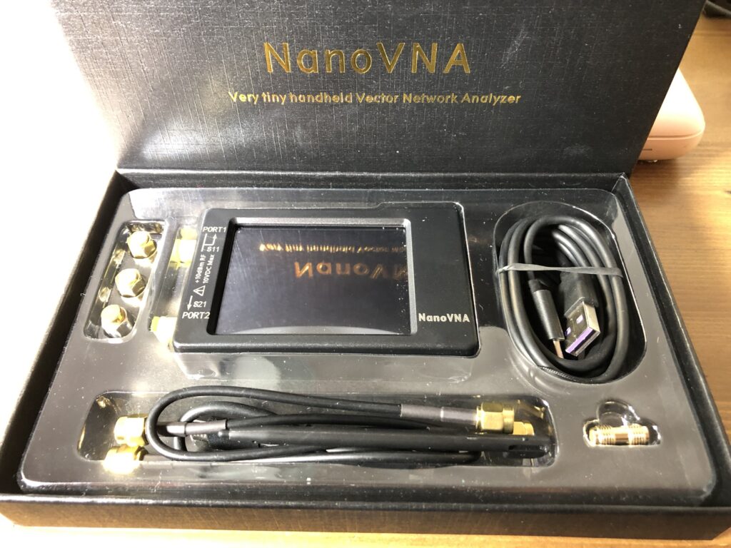
Basically, you get everything you need to get started with this diminutive piece of test gear! As you can see from the photo, the NanoVNA comes with a selection of accessories that are important:
- The items needed to calibrate it.
- Stylus to use on the touch sensitive screen.
- USB-C cable to charge the unit and connect it to a Mac / PC / etc.
- SMA female to female connector.
- 2x SMA cables to interface the unit with the item to be measured.
- Menu layout diagram (not shown).
Additional Equipment
If you are going to use this equipment for UHF measurements, you may want to purchase some higher quality SMA cables, but for everything else, what’s in the box is fine.
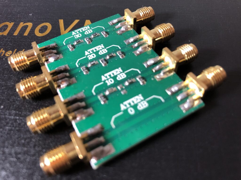
I would also suggest that you are going to need a multitude of adapters to convert the SMA to BNC / PL259 / SO239 / N-type / etc. You may also benefit from buying an attenuator too, which are available at low cost, such as that shown below.
The NanoVNA
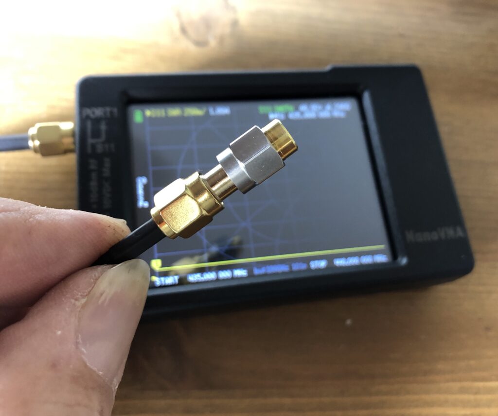
The NanoVNA has three connectors, one of which is the USB-C connection which is used to charge the device, or connect it to a Mac / PC / Android / Linux computer. I use a Mac and the NanoVNA Saver software… if you’re just starting out, I would recommend getting used to the device first, before getting stuck in with the software.
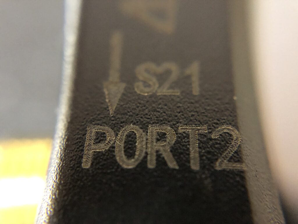
So, in addition to the USB-C, there are two SMA connectors, Port 1 and Port 2. These are the ports that you will connect your device under test (also known as a DUT) to. It’s important to understand what it is that you are attempting to test, so that you select the appropriate port(s) to use.
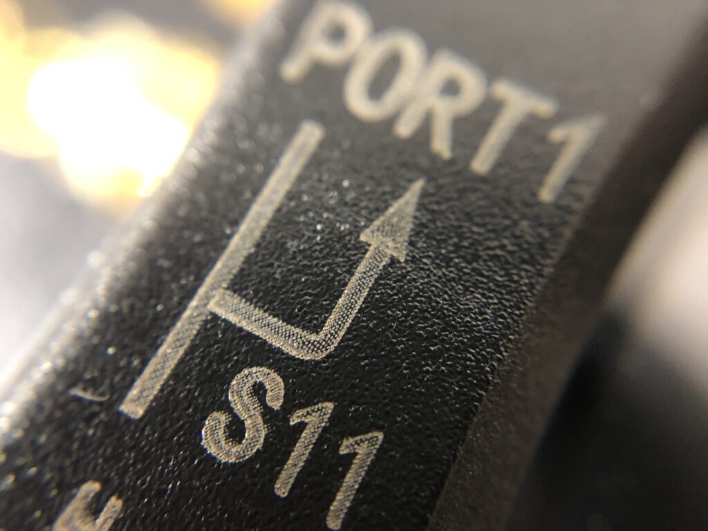
Port 1 sends an outgoing test signal, and then measures the reflected signal.
Port 2 receives an incoming signal.
In some cases, you’ll only use Port 1 (VSWR measurements fall into this category). Other times, you’ll need to connect to both Port 1 and Port 2 (filter analysis, for example).
You’ll also see S11 and S21 being referred to. The first of these tells you that the signal is being measured at Port 1 and the signal is generated at Port 1 – hence S11. The latter signifies that the measurement is taking place at Port 2 but the signal is being generated at Port 1 – hence S21.
On ‘proper’ VNA, you are also likely to get S12 and S22 as well – but on the NanoVNA we’re stuck with S11 and S21. In reality, for the vast majority of uses, this is not a hindrance.
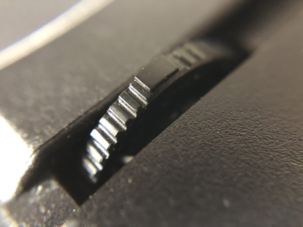
At the side of the NanoVNA, there is also an on-off switch (next to the USB-C connector) and a thumbwheel for selecting menu options. This thumbwheel can also be pressed down to make a selection.
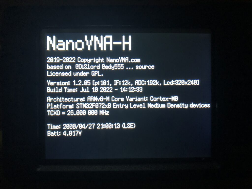
Just a quick note… the NanoVNA is an open source piece of equipment, which means that there are different versions of firmware running the device. You may find that your NanoVNA has some subtle differences than my one, used in these photos. You can see what version of firmware you are running by selecting Config > Version from the menu.
Display & Calibration (S11)
The NanoVNA will need to be calibrated before it can be used, and the equipment to complete this is provided in the box. But before we delve into calibrating it for use, let’s have a look at the display first.
The Display
The main part of the display is taken up by the area that will provide the measurements, but there are areas to the top and bottom, as well as the sides that are also used to provide information or menus.
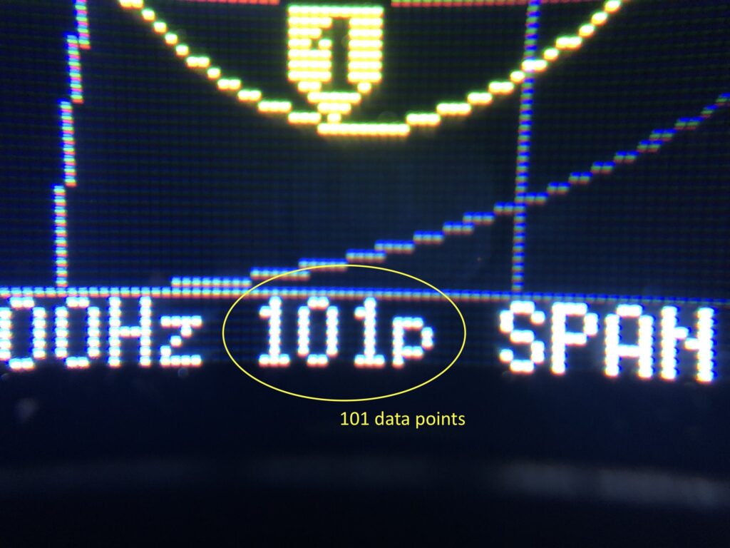
The top of the screen displays information for up to four different traces – these relate to S11 and S21 measurements. The bottom part of the screen displays frequency information and the number of data points selected (the NanoVNA uses up to 101 points).
The right edge of the screen is used for the menu, which you can bring up by tapping the stylus on the screen and then making your selections.
The left edge of the screen provides calibration information.
Calibration
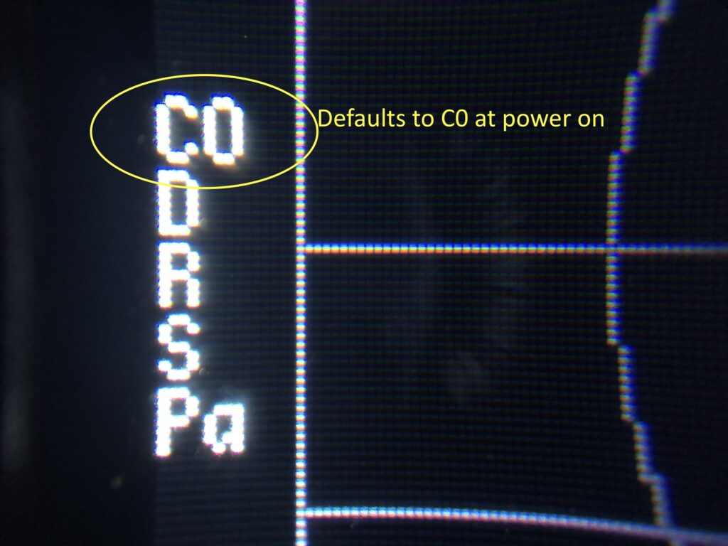
The unit comes with a default, factory calibration, known as C0. When you switch the unit on, this is what the NanoVNA defaults to. Note that this is a capital ‘C’ and not a lowercase ‘c’ – as we’ll see, that has a specific meaning.
When we want to use the device for a particular purpose, it’s useful to ensure that we calibrate it with respect to the frequency (or frequency range) of interest. This will ensure the most accurate results. Depending on the type of measurement, we will need to calibrate the machine appropriately. There are two ‘types’ of calibration:
- If we are using only Port 1 (S11), then we need to calibrate Open, Short and Load.
- If we are using Port 1 and Port 2 (S21), then we will additionally need to include Isolation and Thru calibration too.
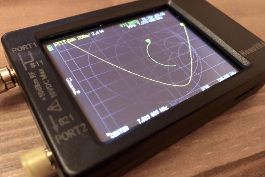
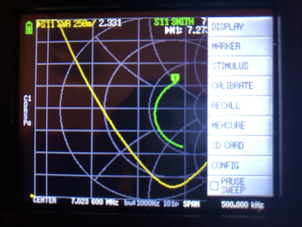
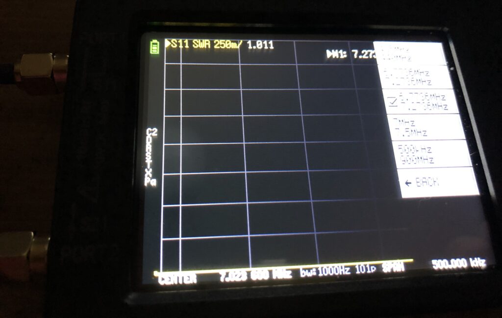
Understanding the calibration is probably made easier by going through a real-world scenario, so let’s start by checking the VSWR of a simple inverted-v dipole for the 40m band. I built this antenna specifically for use with a Pixie transmitter (and the Forty-9er), so I know the frequency of interest is going to be 7023.6kHz. However, rather than just checking one frequency, I’m looking to get some information over a 500kHz span of frequencies, centred on 7023.6kHz.
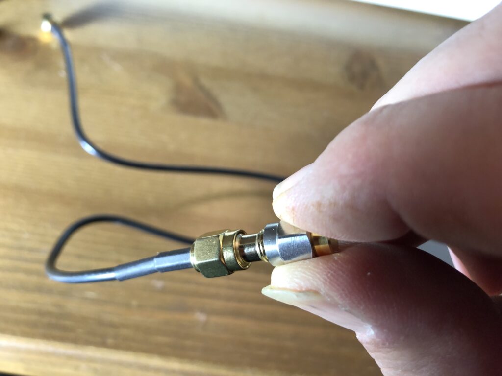
For this calibration, we will only need to use the open, short and load calibrators, the SMA female-female connector and one of the SMA pig-tail leads. It’s highly advisable to always use a lead when connecting items to the NanoVNA as this considerably reduces stress on the SMA connector (which is soldered directly to the PCB).
The first step is to switch the unit on, then set the frequency / frequencies of interest. Tap on the display to bring up the menu, select Stimulus, then Centre. This is the central frequency of the sweep, which in our case is 7023.6. Then select Span and enter 500k.
At this point, can begin the calibration process. Select Calibrate, Calibrate, then connect the open circuit calibration connector to the pig-tail. Now select Open. At the top of the screen you might just see a blue line advancing across, once this reaches the other side, the [open] calibration is complete and the device will be expecting the short circuit connector. Unscrew the open connector, replace it with the short circuit connector and tap Short. Repeat this process for the 50Ω load, then select Done. Remove the load.
At this point, it’s worth saving this calibration (especially if it is one that we are likely to re-use). Click on Save 1. You can now tap on the screen and the menus will disappear; the calibration has been saved to Calibration 1. In normal use, you would now carry out your measurement but as we’re interested in find out a bit more about the calibration, switch off the NanoVNA, then turn it back on again.
We saw before that the unit defaults to C0, but we have saved our calibration to C1. We need to recall this calibration… bring up the menu, select Recall, then select the frequency range you just set.
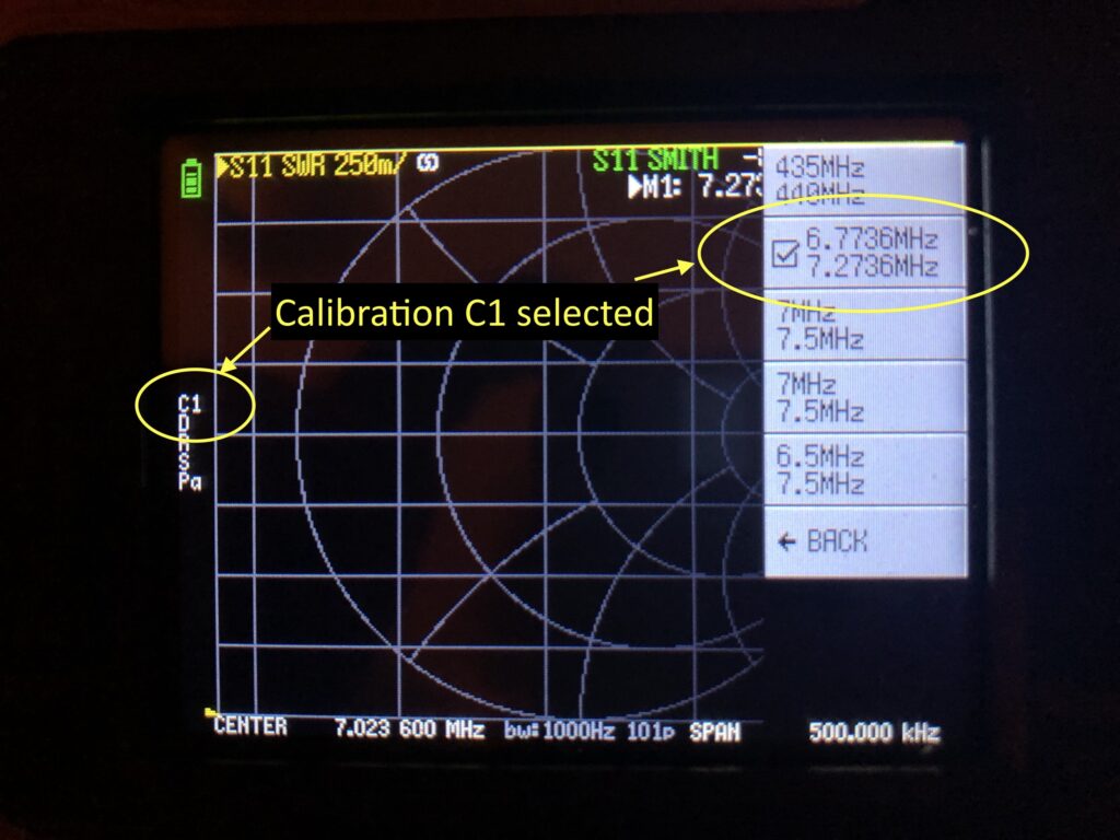
You will now see, on the left hand side of the screen, that the calibration has now changed from C0 to C1. We are now ready to take our VSWR measurements across the frequency range that we’ve just set, which is +/-250kHz either side of the central frequency of 7023.6kHz (or 6773.6 – 7273.6kHz). But what if we wanted to now test a slightly different range, say starting at 6320kHz?
Whilst we can re-calibrate, in this case, it’s probably okay for our purposes just to reset the start and stop stimulus to the newly desired range. However, we’ve not calibrated it for these specific frequencies and when this happens, you’ll note that C1 changes to c1. This shows that the device has been calibrated but not for the exact frequencies now being used.
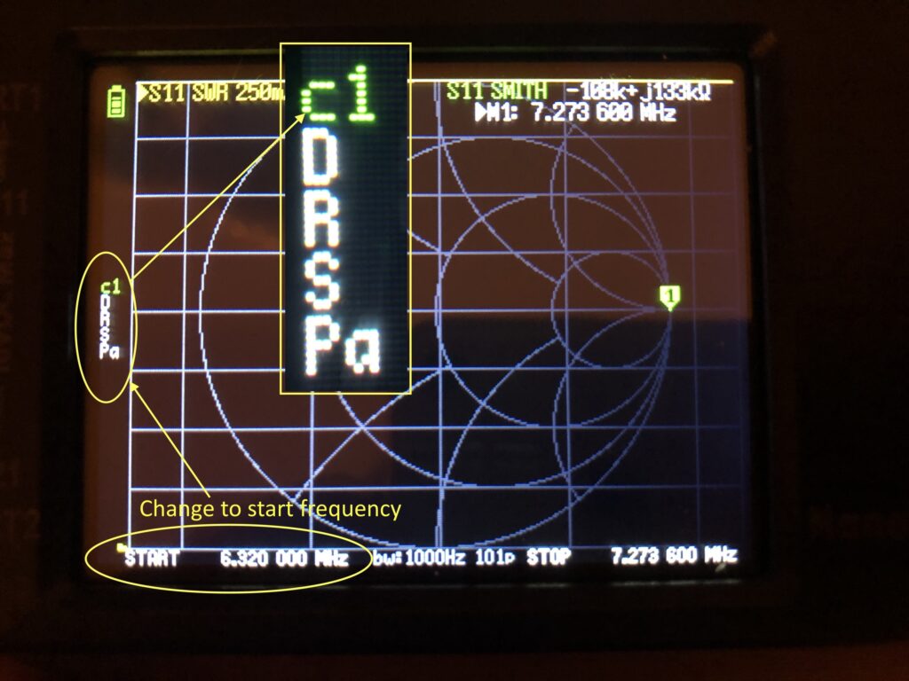
What of the other letters under the C1 / c1 though? The D, R and S relate to the type of calibrataion:
- D relates to ‘directivity’ using the 50Ω load
- R is related to ‘reflection’ using the open circuit connector
- S stands for ‘source match’ using the short circuit connector
- Pa relates to automatic power level setting for calibration
Display and Calibration (S21)
When using the S21 port (ideal for filter analysis), we’re going to be measuring the transmitted signal from Port 1, on Port 2. There are two extra steps in completing this calibration:
- Isolation
- Through
Through Calibration
To complete this calibration, you will need to connect Port 1 and Port 2 together using the supplied cables and the female-female SMA connector.
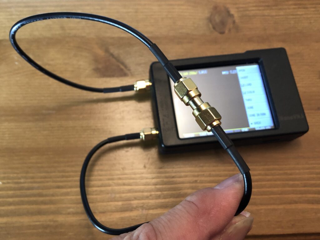
If you are after the best calibration, make sure you use both the cables, as shown in the image – don’t be tempted to just short the ports with one cable (remember, you will be connecting the filter across the ports using both cables).
Once you’ve connected the ports together as shown, tap on ‘Through’ in the Calibrate menu.
Isolation Calibration
Done properly, this calibration should be done with a 50Ω load on each port. However, we only get one 50Ω load with the kit, so this must be connected to Port 2 (leave Port 1 open circuit with no connector).
With this done, tap on ‘Isolation’ in the Calibrate menu.
Display
You will notice on the main display, that there are couple of new letters on the left hand side of the screen. These letters ‘T’ and ‘X’ relate to completing the Through and Isolation calibration sequence.
You are now ready to use the NanoVNA to test and analyse using Port 2 for measurements.
Testing Filters
The NanoVNA is a great tool for analysing filters, using the S21 port. As we’ve seen, this will transmit a signal from Port 1, with the response measured on Port 2. By setting our start and stop frequencies, we can analyse the response curve of a filter.
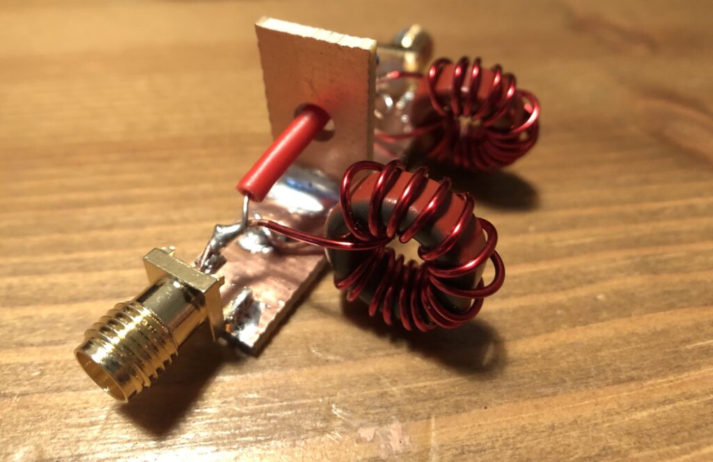
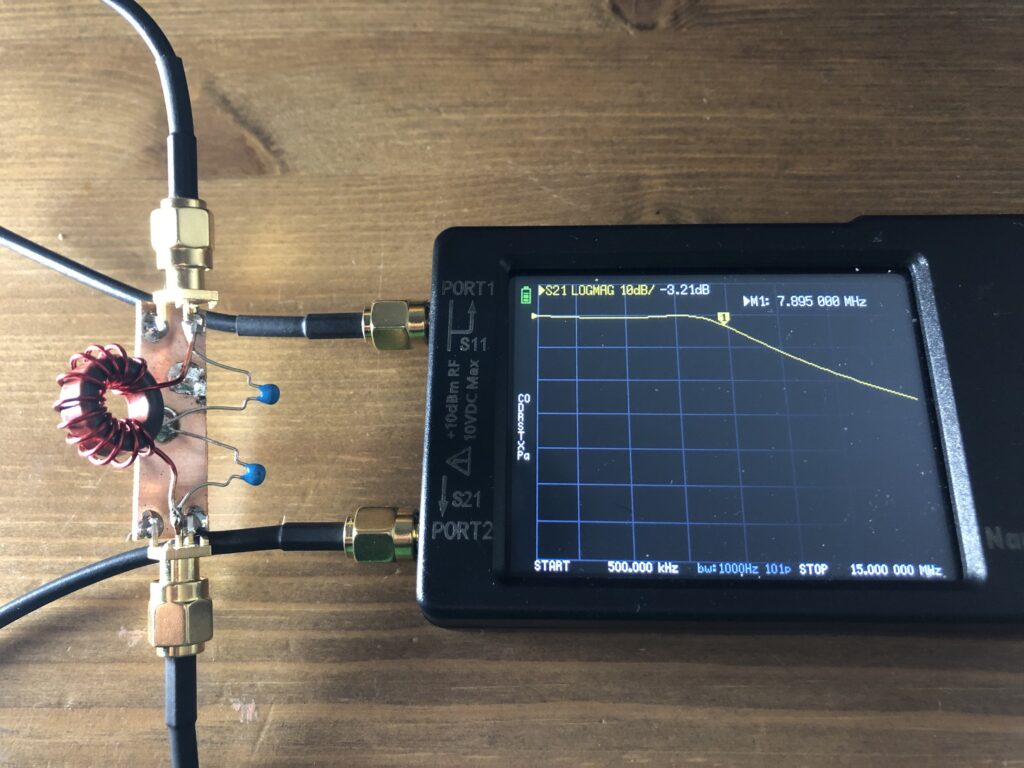
We’ll start by building an experimental high-pass filter, using 15 turns of 22AWG enamelled wire on a T50-2 toroid (x2), and a 1nF capacitor.
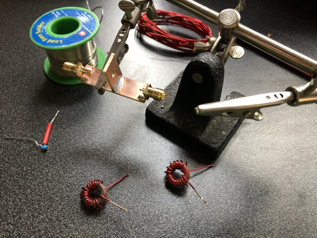
This filter was actually built to complement a low-pass filter that I had already built for testing with the NanoVNA, so that we could put them together as a band-pass filter.
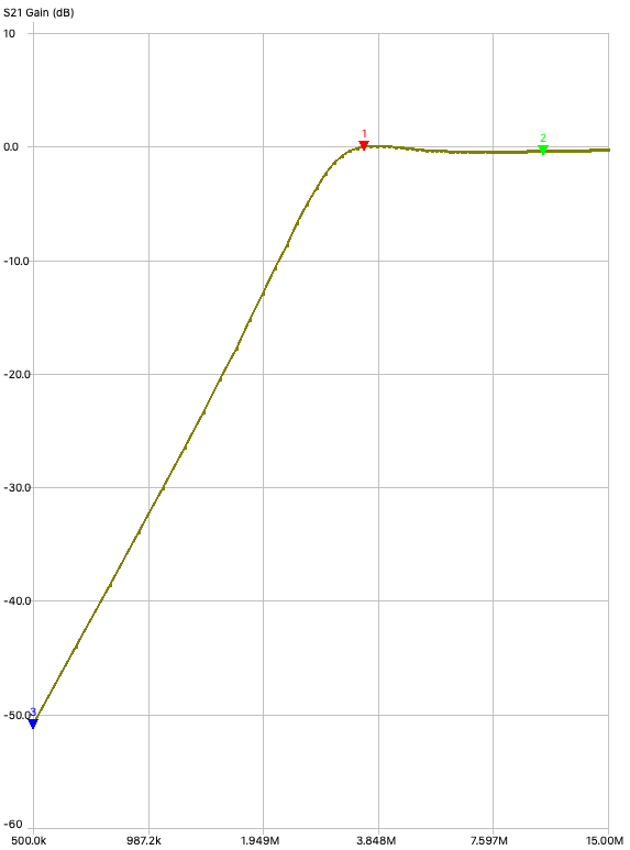
After calibrating the NanoVNA, with a start frequency of 0.5MHz and a stop frequency of 15MHz, we can connect the filter between Ports 1 and 2. Set a single trace to display S21 logmag and you can see the response curve for this filter.
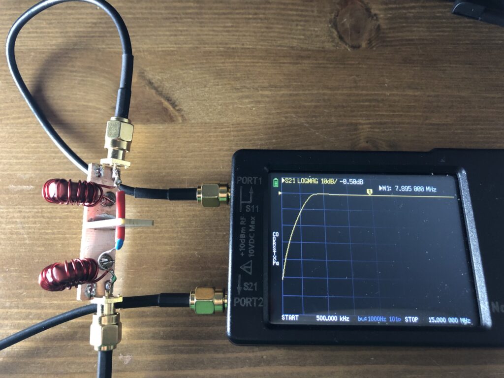
The filter appears to be acceptable as a high-pass filter from the 80m band upwards, with a steep fall-off below 3MHz.
The previously built low-pass filter was also analysed, this giving a much softer roll-off of higher frequencies.
The low-pass filter uses a single T50-2 toroid with 13t of 22AWG wire, and two 1nF capacitors. Putting the low-pass and high-pass filter together should give us a band-pass filter that would cover 80m and 40m… let’s test that out…
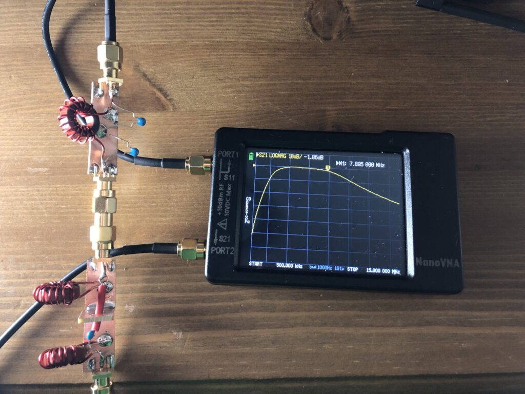
As we can see, connecting these two filters together seems to provide a band-pass filter and by moving the marker along, I can estimate that the -6dB points are around 2.35MHz on the lower side, and 9.9MHz on the upper side. The main pass band is fairly flat across the 80m and 40m bands.
Analysis Using NanoVNA Saver
NanoVNA Saver is an add-on piece of software that complements the NanoVNA, adding some useful functionality. In this article, we’ll look at how we can use this software to analyse the band-pass filter that we used in Part 4 of this series.
In Part 4, we estimated that the -6dB points of the band-pass filter were approximately 2.35MHz and 9.9MHz, but let’s see how close we got…
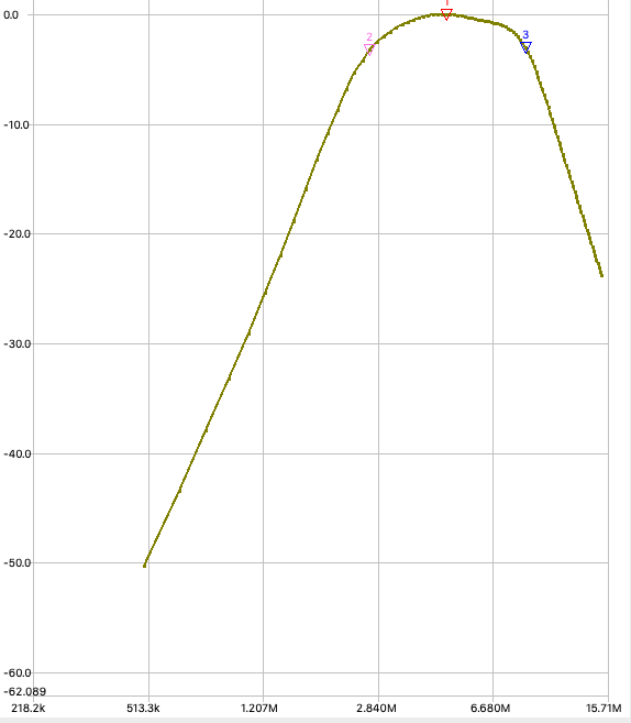
The sweep was set using the same as before (0.5MHz – 15MHz) and we can set the graph to display frequency with a logarithmic scale, as above. Marker 1 is the centre of the pass band, with markers 2 and 3, at the -3dB points.
Within NanoVNA Saver is a button that allows you to automatically analyse the filter, in this case as a band-pass filter (but other options are available from a dropdown list). Analysing the filter results in a pop-up window detailing the information gleaned…
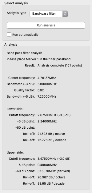
As we can see, the -6dB points of the filter were actually at 2.24MHz and 9.49MHz – relatively close to our estimate direct from the NanoVNA display. We can also see that our filter bandwidth is 7.25MHz at the -6dB points, or 5.8MHz at the -3dB points. The filter is centred around 4.76MHz and means that we can comfortably cover the 80m and 40m bands.
NanoVNA Saver
In part 5 we introduced the complementary software, NanoVNA Saver. This provides additional functionality to the NanoVNA unit and is worth downloading (note that the following images were taken using a MacBook running the NanoVNA Saver application).
Connecting The NanoVNA
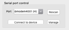
Using the USB cable supplied, connect the NanoVNA to your PC/Mac (I tried Linux, but couldn’t get it to work!). Switch the unit on then start the application. You will need to ensure that the correct port is being used on your machine, and then click on Connect to device.
You can now connect your device under test, ready to be analysed. In this example, I used the high-pass filter that I’d built earlier in this series.
Sweep Settings
By default, the NanoVNA makes a sweep of the frequencies that are set in the application. This sweep is made up of 101 data points.
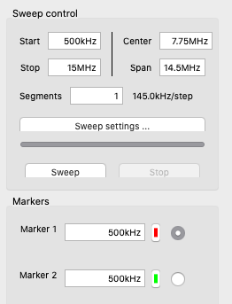
This is fine but be aware that when sweeping a wide range of frequencies, there can be a large step between each data point; this reduces accuracy. In the image above, I’ve set the sweep to start at 0.5MHz and stop at 15MHz. This results in a 145kHz step between each data point.
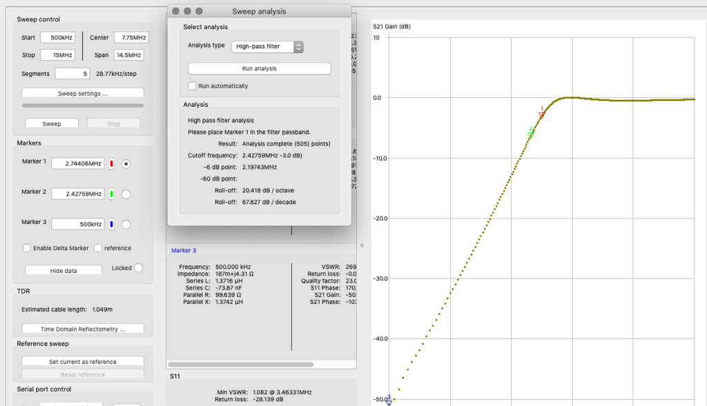
We can improve this by altering the Segments setting… changing this to 5 segments reduces the step to just under 30kHz. Essentially the 0.5MHz to 15MHz sweep is split into 5 parts, meaning there are now 505 data points covering the desired sweep range.
The NanoVNA Saver application defaults to a single sweep (i.e. measurements are taken just once for each data point). However, we can change this so that more than one sweep is completed and the results are averaged.
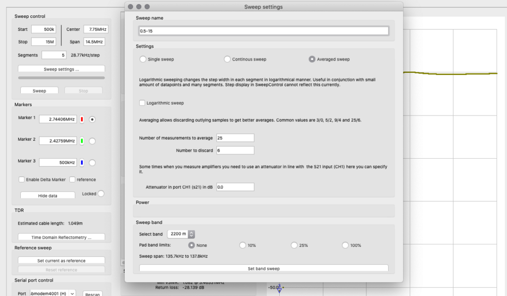
We achieve this by clicking on Sweep settings…, which opens up a new window. Select Averaged Sweep, then set the Number of measurements to average to the required setting (examples are given in the window) and Number to discard. This will get rid of outliers that may skew the results.
The frequency to sweep has already been set, as has the number of segments. You can just close this window (no need to click on Set band sweep in this window).
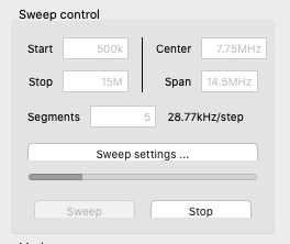
The progress bar will show the progress made by the application – be aware this may take a little time!
Sweep Setting Results
We make these adjustments in a bid to improve the accuracy of our results. So let’s see what difference it makes. Running the high-pass filter analysis tool with default setting gave the following results:
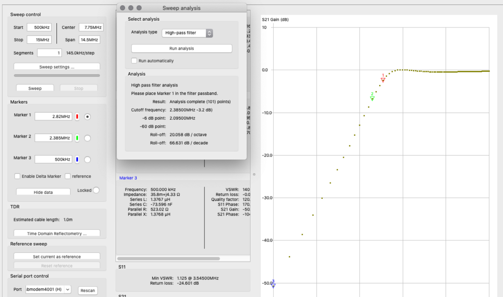
The cutoff frequency was given as 2.385MHz, with the -6dB point at 2.095MHz (default settings).
After amending the sweep settings (5 segments), the cutoff frequency was given at 2.427MHz, with the -6dB point at 2.197MHz.
Changing The Graphical Display
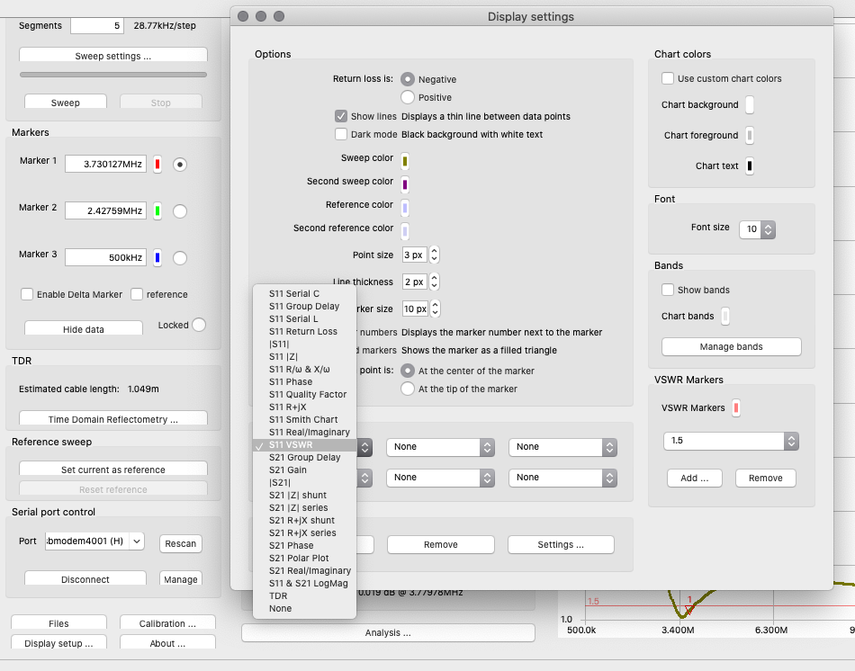
You can select the graph(s) that you wish to display by clicking on the Display setup… button. This brings up a pop-up window that will allow you to make various choices about how you wish the graphical area to be displayed. It also allows you to select which graph(s) should be displayed. In the image below, the VSWR graph has been chosen.
Once this is set, the display will change and you can close this pop-up window to display the graph…
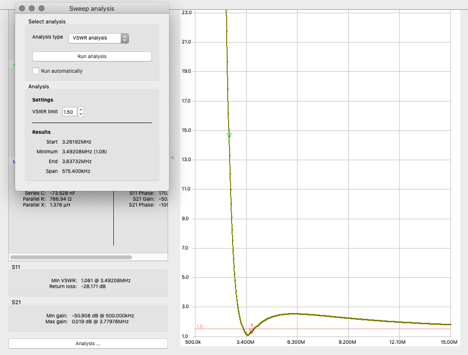
Previously, the analysis tool had been used to look at the response curves of the filter, but we can also analyse other metrics; in the image above the VSWR has been analysed and provides the frequencies at which the VSWR reaches 1.5:1.
Additional Functionality
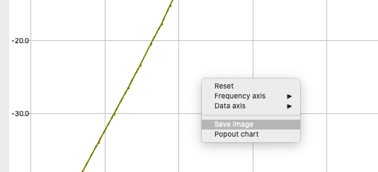
NanoVNA saver also allows you to save the graph as a picture file. Ctrl+click (note: Mac OSX) in the graph area displays a pop-up menu, select Save image to save the graph.
The saved graph is shown below: